Table of Contents
- 3.1. Advanced Model Explorer
- 3.1.1. Entity table
- 3.1.1.1. Workflow metadata
- 3.1.1.2. Worfklow inputs and outputs
- 3.1.1.3. (Slight digression) - Some facts about using MIME types in Taverna
- 3.1.1.4. Connecting workflow inputs to processors
- 3.1.1.5. Processors (Top level node)
- 3.1.1.6. Individual processor nodes
- 3.1.1.7. Data link nodes
- 3.1.1.8. Control link nodes
- 3.2. Interactive Diagram
- 3.3. Workflow diagram
- 3.4. Available services
- 3.5. Enactor launch panel
The main section of the AME shows a tabular view of the entities within the workflow. This includes all processors, workflow inputs and outputs, data connections and coordination links. Some items may be expanded to show properties of child items such as alternate processors and input and output ports on individual processors. In general the right click menu on an entity will expose at least 'delete from workflow' functionality and may provide more.
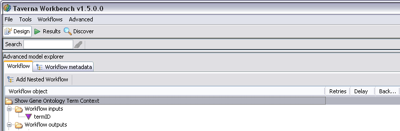
By selecting the name of the workflow at the top of the AME, a new tab 'Workflow metadata' becomes available:
Selecting this tab shows the workflow metadata display:
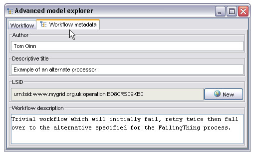
This panel allows the user to enter an author name, descriptive title and longer textual description. The Life Science Identifier (LSID) field is not manually editable, instead the 'New' button will connect to whatever LSID authority is configured in the mygrid.properties file and ask for a new LSID suitable for a workflow definition. This then provides a globally unique identifier for the workflow definition (as opposed to workflow instance, each instance of a workflow within the enactor also has a unique ID but this isn't it). The original AME view can be restored by selecting the 'Workflow' tab.
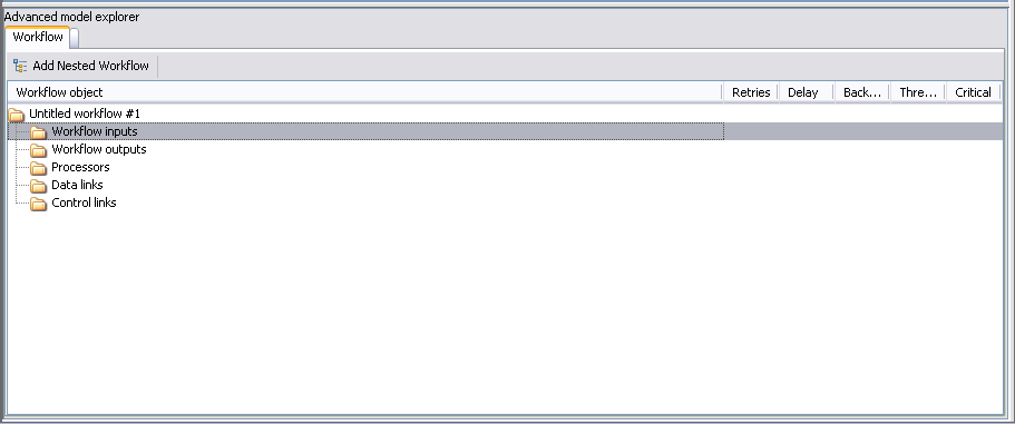
The 'Workflow inputs' and 'Workflow outputs' nodes are used to create, respectively, workflow inputs and outputs. A new input or output can be created by right clicking on the text and selecting 'Create new input...' or the obvious corresponding option for outputs. This then displays a text dialogue into which the name of the new workflow input or output should be entered. Once created, the name can be edited by triple-clicking on the name and editing in the normal way.
Once a workflow input or output has been created it can be further specified by selecting the input or output node in the tree and opening the newly available tab, 'Metadata for [input or output name]'. This tab two sub-tabs for different parts of the input description. These tabs allow entry of a free text description (for workflow inputs this is shown in the workflow launch panel so is a good place to put information which users of the workflow would need to populate the inputs) and tagging of the input or output with MIME types. The latter is particularly important for workflow outputs as it drives the selection of renderers within the result browser. The description panel is self explanatory, the MIME type entry is shown below:
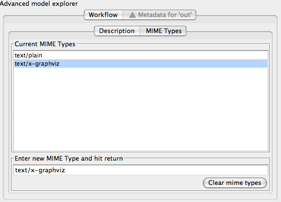
The large button at the bottom right of the panel will completely clear the MIME type list. Outputs and inputs in Taverna can have multiple MIME types - these are regarded as hints to the rendering system rather than being prescriptive computer science formal types. To add a new MIME type the user enters the type into the text box and hits the return key, it then appears in the type list.
The following is a list of the MIME types currently recognized by renderers in Taverna's result browser, this list is useful to know when annotating workflow outputs for obvious reasons which is why it appears here rather than elsewhere.
text/plain=Plain Text
text/xml=XML Text
text/html=HTML Text
text/rtf=Rich Text Format
text/x-graphviz=Graphviz Dot File
image/png=PNG Image
image/jpeg=JPEG Image
image/gif=GIF Image
application/zip=Zip File
chemical/x-swissprot=SWISSPROT Flat File
chemical/x-embl-dl-nucleotide=EMBL Flat File
chemical/x-ppd=PPD File
chemical/seq-aa-genpept=Genpept Protein
chemical/seq-na-genbank=Genbank Nucleotide
chemical/x-pdb=Protein Data Bank Flat File
chemical/x-mdl-molfile
At the present time the behaviour for textual types is to render them either as plain text or as an XML tree for text/xml, a rendered graphical view for text/x-graphviz and Java's best attempt at rich text or HTML for the respective types. The various 'chemical/...' types are currently rendered using SeqVISTA, another project we integrated recently, this allows a very attractive view of sequence data in particular. The exception is the chemical/x-pdb which uses the new Jmol based renderer. All image types are rendered as images, which is pretty much what you'd expect.
MIME types are also used to attempt to guess the appropriate file extension when storing results to a file system tree, this is currently the only reason to tag an output as application/zip. Taverna has no other understanding of zip files
You can add multiple mime types to a workflow output port (to be used by the output renderers) by selecting the output and going to "Metadata for 'myoutputport'" - under "MIME types", eg for SVG add: image/svg+xml This should enable the SVG renderer for the output port. You might need to right click on the value in the left hand column and select "SVG" instead of "Text".
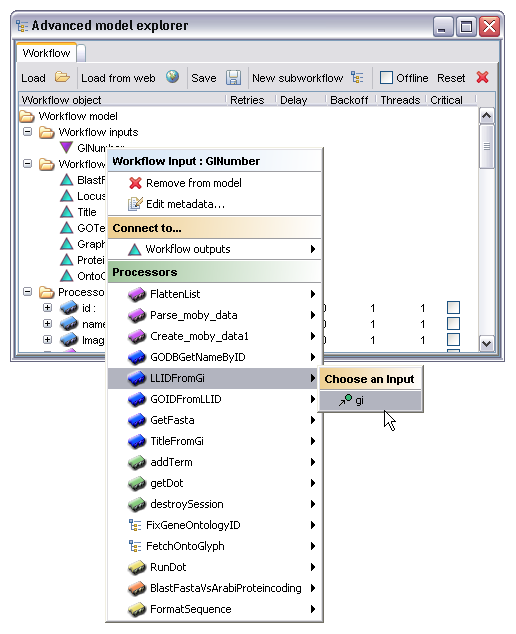
Workflow inputs may be linked to the inputs of processors within the workflow (or directly to workflow outputs) by right clicking on the particular workflow input and selecting the target from the drop down menu, either selecting a workflow output directly or selecting a processor then the workflow input within that processor. Conceptually links in Taverna always link from an output to an input, this is slightly confusing in the sense that workflow inputs are, as far as the workflow itself is concerned, also outputs - they produce data. In a similar way workflow outputs are in fact inputs, they consume data and manifest it to the outside world in the form of workflow results. The image below shows a workflow input being linked to the input of a processor:
The processors in Taverna are the primary components of the workflow. They are the entities responsible for both representing and ultimately invoking the tasks from which the workflow is comprised. In addition to allowing the manipulation of the individual processors this section also exposes a summary of all the remote resources used by the workflow, this can be shown by selecting the 'Processors' node and opening the 'Remote resource usage' tab that appears :
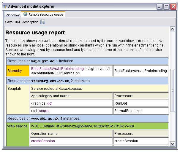
This display summarizes remote resources by host, giving a quick overview on which tools from which institutes the workflow uses. This report can be saved in HTML form and also includes the description, author, title and LSID if present defined in the workflow metadata. The intention is that between this and the workflow diagram much of the description you'd need for a paper or poster is auto generated.
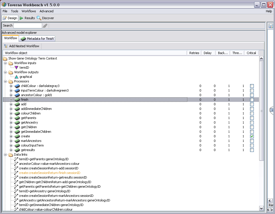
Each processor in the workflow is represented by a processor node in the AME. These nodes can be expanded to show the inputs and outputs of that particular processor, selected to enable a tab containing metadata about the processor or double clicked on to edit the name of the processor.
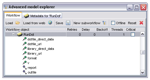
In this case the processor is one based on Soaplab (indicated by the yellow icon colour) and has many inputs and two outputs. The input and output names are shown as children of the processor, with different icons for inputs and outputs. Selecting the 'Metadata for 'RunDot'' tab shows the following information:
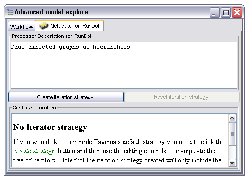
The metadata panel contains a free text description (which may or may not be populated from the service by default) and an editor for the iteration strategy. More details of the iteration system can be found in the iteration section, it will not be discussed further here. Return to the standard AME view by selecting the 'Workflow' tab.
Processors are instances of components available in the 'Available Services' panel, and are selected from there. See the Available Services section for more information.
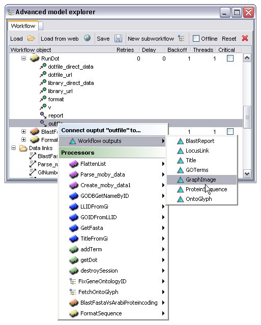
The port nodes under each processor node are used to connect the outputs of processors either to the inputs of other processors or to workflow outputs. This is achieved by right clicking on the output port node and selecting either a workflow output (as shown in the case below) or by selecting a processor then the appropriate input within that processor.
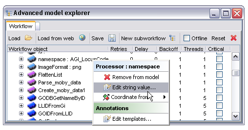
Some processor types may expose additional editors. For example, the processor type which emits a string constant has a very simple editor which allows the user to change the string it emits, the beanshell processor has a more sophisticated one providing a lightweight script editing environment and the nested workflow processor uses another instance of the AME as its editor. These editors, if available for the selected processor, are accessed from the right click menu on the processor node itself. The exact behaviour depends on the processor type :
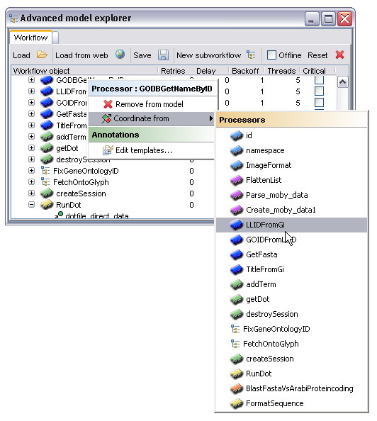
It is sometimes required to prevent a processor running until some condition is true. The most common (and in fact the only currently supported) condition is that processor A should only run when processor B has completed successfully. This constraint is created by right clicking on the processor node and selecting a target processor from the 'Coordinate from' menu. The semantics of this constraint are that the processor first selected will only start running once the processor selected from the menu has completed. It's worth noting that in the case where processor A is feeding data to processor B in some way this temporal condition is implicit, an explicit statement of the condition is only required where there is no other form of linkage between the processors. In the example below the processor 'GODBGetNameByID' will only run when the processor 'LLIDFromGi' has completed:
Each processor in the workflow has its own settings for fault tolerance. These settings include the ability to retry after failures and to fall back to an alternative or set of alternative processors when all retries have been exceeded. The state machine governing this process is shown below:
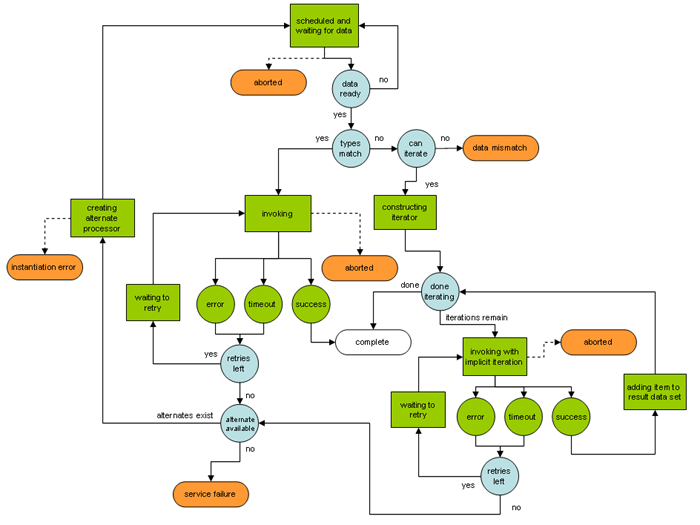
The main point to take from this diagram is that during iteration, individual iterations will be retried, but that if all retries are exhausted during any single iteration the entire process will be rescheduled with an alternate. So, if there are two hundred iterations and the last one fails the entire set of two hundred will be re-run on the first alternate, assuming there is one available.
Initial configuration of the retry behaviour for each processor is done through the columns to the immediate right of the processor nodes in the AME main work area. By double clicking on these the user can change values for, from left to right, 'Retries', 'Delay' and 'Backoff'. These are the basic retry configuration options and have the following effects.
Retries - the number of times after the first attempted invocation that this processor should be run. So, if set to 1 there will be one retry after the first failed invocation.
Delay - the time delay in milliseconds between the first invocation failing and the second invocation attempting to run. Time delays can often be useful in cases where resources are less than optimally stable under heavy load, often in these cases simply waiting a second or two is enough to get a successful result.
Backoff - a factor determining how much the delay time increases for subsequent retries beyond the first. The time between attempt 'n' and 'n+1' is determined by multiplying the delay time by the backoff factor raised to the power of 'n-1'. So, if this value is set to 2 and the initial delay set to 1000 there will be a pause of one second between the first failure and the first retry, then should that in turn fail there would be a delay of 1000 x 21 = 2000 milliseconds or two seconds, the next would be four etc. Specifying a backoff factor reduces the load on heavily congested resources and is generally a good idea - the default value of 1 specifies no backoff, the delays will not increase between retries.
The 'Critical' checkbox determines what should happen if all retries and alternates have failed. If left unchecked the workflow will continue to run but processors 'downstream' of the failed processor will never be invoked, if checked then any failure here will abort the entire workflow.
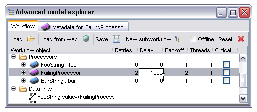
The image below shows the user editing the delay factor for the processor 'FailingProcessor'. In this case the processor will retry twice after the initial failure, waiting first one second then two.
Once all retries have been used up without any successful invocation the processor concerned will fail, and either silently abort all downstream processors or abort the entire workflow, depending on whether the 'Critical' box is ticked. It is often possible, however, to have an alternative processor or list of processors which perform the same task, perhaps on a different server, and Taverna allows the user to explicitly state this in such a way that the alternate is used in place of the main processor when the latter has failed. To configure alternate processors the user expands the node for the main processor by clicking on the expand icon to the left of the processor icon. This then shows the inputs and outputs of the processor as before but also shows any defined alternates. An example of this display is shown below with the alternate fully expanded as well:
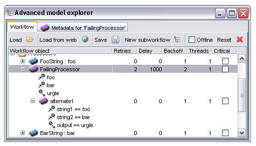
Note that the alternate has its own definable parameters for 'Retries', 'Delay' and 'Backoff'. The behaviour here is that once the main processor has failed and exceeded all retries the alternate is scheduled in its place, using the alternate's parameters for fault tolerance features.
As alternate processors may well not have the same names for inputs and outputs it is often necessary to explicitly state that a particular port in the primary processor is equivalent to another in the alternate. This is done by selecting the port in the alternate and right clicking, then selecting the port in the primary processor for which this is an equivalent. In cases where the alternate processor has port names which match those in the primary Taverna will automatically create a default identity mapping.
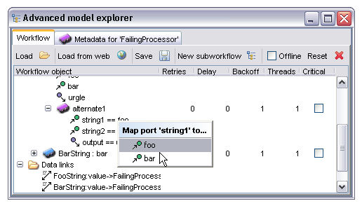
In this particular case the port with name 'string1' in the alternate is being mapped to the input port named 'foo' in the main processor.
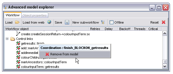
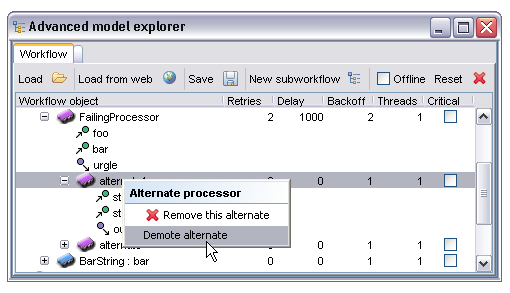
Multiple alternates may be specified, if this is the case the order in which alternates will be used can be changed by right clicking on the alternate node and selecting 'Promote alternate' or 'Demote alternate' as appropriate. Alternates may also be removed from this menu:
The 'Threads' property determines how many concurrent instances of the processor should be used during iteration. This property only ever has any effect therefore if there is some kind of iteration occurring over the input data. To understand why you might want to change this property, consider the following example.
Suppose there is a service which takes one second to run. On the face of it starting five instances of this service simultaneously will take exactly the same time as running five in series, assuming here that there is a single CPU backing the service. There is, however, another issue to consider; services invoked over a network link incur an additional time cost called latency - this is the time taken for the data to be transported to and from the service, the time to set up any network traffic etc. If we have this one second process but in addition half a second before and after to send the data clearly there will be a one second pause on the service end between iterations corresponding to the time to send the result back and for the enactor to send the next input data item. If, however, multiple threads run concurrently the enactor is sending data at the same time as the service is working on the previous input - the service in this case never has to wait for the next input item as it has already been sent while it was working on the previous one.
In the case of the service described above, running five iterations in series would take 5 x (0.5 + 1 + 0.5) = 10 seconds. If we were to run all five in parallel the time taken is 0.5 + 5 x (1) + 0.5 = 6 seconds, the half second latency occurs at the start and end of the entire process rather than per iteration. Clearly under these conditions running multiple worker threads is beneficial.
The other case where this is a reasonable thing to do is where the service is backed by some significant multiprocessor compute resource such as a cluster. If we were to send tasks in series the cluster would only ever have one job running at any time, whereas a parallel invocation would allow the workflow to saturate the cluster, running all nodes in the cluster at full capacity and completing massively faster. If our example above were run on a five node compute cluster the total time would actually be 0.5 + 1 +0.5 = 2 seconds, the five jobs all running simultaneously on different units within the cluster.
Taverna sets a limit on the maximum number of threads for each processor type. It is also generally a good idea to check with the administrator of the service concerned before hammering it with massively parallel requests, not all services can take this kind of load!
Each data link (between workflow inputs, processors and workflow outputs) in the workflow appears under the 'Data links' node in the AME. This display is largely informational although data links may also be deleted from the right click context menu. Note that any data links connected to a processor are deleted if that processor is also deleted. There are no 'hanging links' in a workflow model.
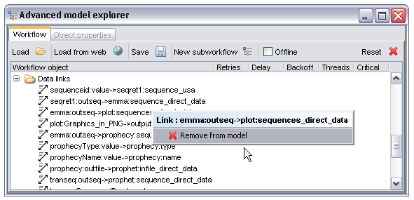
Naming for the data links is in the form of the processor name and port name for the output or data source, separated by a colon, then an arrow and the same syntax for the sink or input port it links to. In the case of workflow inputs and outputs there is no processor name, just the name of the output or input.
As with the data links these are primarily for information but also allow removal of individual control links. The naming syntax consists of the processor acting as the gate condition, two colons then the name of the processor being controlled by it. So, 'foo::bar' represents a condition stating that 'bar' may not start until 'foo' has finished.